Personal project · Data science · 2026
Can a model learn a structured representation of a world from pixels alone?
No labels. No reward. No rules handed to it. Just a stream of images — and the task of predicting what comes next. This is the bet of world models, and this is what this project explores.
5×5 grid · 4 directions · walls stop movement · no target, no score.
You understood that in seconds. Can a model figure it out just by watching images and actions?
Starting point
LLMs manipulate text. The world is not text.
In early 2026, Yann LeCun — Turing Award recipient, founder of AMI Labs — made a sharp argument: large language models are impressive, but fundamentally limited. They predict the next token in a sequence of words. But intelligence isn't about tokens.
"The world is far more complex than language. As humans, we tend to think an entity is intelligent if it manipulates language — but we are misled. Language is a sequence of discrete symbols. The real world is far more complex, and understanding it requires completely different techniques. The question is: how do we get machines to learn the world by observing it, the way a young child does — or even a house cat?"
Yann LeCun — France Inter, L'invité du 7h50, 10 mars 2026 ↗
His answer is an architecture called JEPA — Joint Embedding Predictive Architecture. In March 2026, his team published LeWorldModel, a concrete implementation of this idea, trainable on a single GPU.
This project is an attempt to implement that idea from scratch — on a minimal simulated world — and understand it from the inside. Not by reading. By building.

The architecture
JEPA — predict in the abstract, not in the pixel
The core idea is called JEPA: Joint Embedding Predictive Architecture. It rests on two components that train together.
The encoder takes an observation of the world (an image) and compresses it into an abstract representation called a latent vector — a point in a low-dimensional space that captures the essence of the situation. The predictor takes that latent vector and an action, and must anticipate the latent vector of the next state.
The key: the system is not trained to reconstruct images. It is trained to predict in latent space. The encoder must produce a representation the predictor can anticipate. They improve together.
The encoder ϕ is shared between both observations. The loss L₂ brings ẑt+1 (predicted) closer to zt+1 (real) in latent space.
What is elegant about this approach: the system never learns to reconstruct an image. It learns something deeper — a representation of the world that is useful for predicting. Nothing superfluous. Everything functional.
The main risk is called representation collapse: if the encoder maps everything to the same vector, the loss drops to zero — without learning anything. LeWM solves this with a regularizer called SIGReg, which forces latent representations to follow a Gaussian distribution.
The experiment
A 5×5 grid. One agent. Four actions.
We don't write an algorithm that understands the game. We don't give the model any rules. We simply show it images — and let it figure out the rest on its own.
The world
A 5×5 isometric grid. An agent that moves in four directions. No target, no obstacles, no reward signal. The model only sees raw pixel images — 128×128 grayscale — like the one below.
Each training example is a transition: two images and one action. That's literally all the model ever sees. Try it — pick an action below:
Before
Action
After
Pick an action to generate a transition.
50,000 of these transitions. No labels. No coordinates. No rules.
Just pixels — and one of four possible actions.
Dataset & training
The model observes 50,000 transitions — pairs of (image before action, action, image after) — and tries to learn the dynamics from that alone. That's 100,000 images of 128×128 pixels in total.
The model is a ViT-Tiny encoder — a Vision Transformer that reads 128×128 grayscale images — paired with a Transformer predictor conditioned on actions via adaptive layer normalization (AdaLN).
Training
Watch it learn.
200 epochs on 50,000 transitions — these are the real loss values from the actual training run. GPU goes fast. CPU goes slow.
ViT + Transformer
What building this actually taught me
Three things that didn't work — and why.
This is not a research paper. It's an engineering account. The interesting part is not the final numbers — it's what broke along the way.
The model encodes what's easiest, not what's useful.
In an earlier version, the target position was visible in every image. The model learned to encode it perfectly (R²=0.99) — and ignored the agent completely (R²=0.08). The target never moves during a transition: it's the trivial shortcut. Fix: remove the target from the rendered observation. Lesson: always probe what the model actually learned before concluding training worked.
λ=0.1 collapses. λ=10 works.
The paper uses λ=0.1 for SIGReg. On this simple environment, that's not enough — the model collapses to a constant vector (std=0.0007). A simple world makes collapse too easy a solution. The regularizer must be strong enough to make collapse more costly than learning. The right λ is not universal — it depends on the complexity of the environment.
L2 distance in R¹⁹² is not a metric for position.
SIGReg spreads all 192 latent dimensions uniformly (variance ≈ 1 each). Position occupies only 2 of those directions. The remaining 190 dominate the L2 norm — two distant grid positions can be arbitrarily close in latent space. Fix: train a linear probe to decode position explicitly, and plan using decoded coordinates rather than raw L2.
Reading the model
The model lives in 192 dimensions. Let's look inside.
After training, each observation is compressed into a vector of 192 numbers — the model's internal representation of what it sees. That's the latent space: a 192-dimensional world that only the model inhabits. We can't visualize it directly. So we have to find indirect ways to read it.
Projection — PCA
The first tool is PCA — Principal Component Analysis. The idea: find the two directions in 192-dimensional space that carry the most information, and project everything onto them. Like flattening a sculpture into a photograph. You lose detail, but the structure becomes visible.
Here, the two main directions explain 30% + 22% = 52% of the total variance. That's a lot for just 2 dimensions out of 192 — it means the latent space has strong, concentrated structure. And when you look at the projection:
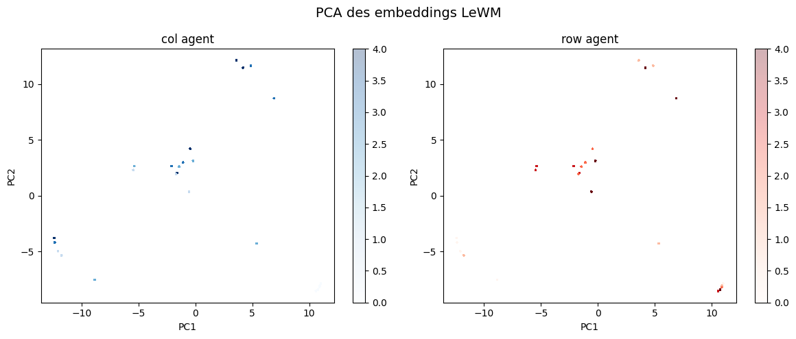
192 dimensions projected onto 2 — colored by agent column (left) and row (right).
Variance explained: PC1=30.0%, PC2=22.0%
5 colors per graph (one per column, one per row) — but look closer: each color contains 5 sub-clusters. 5×5 = 25 positions.
→ tap to zoom and count
25 clusters — one per cell of the 5×5 grid. The model spontaneously organised its internal space to mirror the physical layout of the world. Nobody told it the grid had 25 cells. Nobody told it positions existed. It figured that out on its own, just from images and actions.
Linear probe — reading the model's mind
PCA shows structure, but doesn't measure it precisely. For that, we use a linear probe: a very simple tool — a linear regression — that we inject directly into the model's internal representation, and ask: "can I read the agent's position from this vector?"
Think of it as a scalpel. We open the model at one layer, extract the 192-dimensional vector, and try to decode the (column, row) coordinates from it using only a straight line. No neural network. No trick. Just a linear fit. If it works, it means the information is not just present — it's cleanly organised.
R²=1.0 on both axes means a perfect linear fit. The model encoded position so cleanly that a straight line is enough to read it back — from a representation it built entirely without supervision, without ever seeing a coordinate.
These results should be interpreted in the context of a very simple environment. High scores here do not imply robustness.
So: the model learned something. That something is structured. And we can read it — not by opening the weights and staring at numbers, but by probing the representation with a simple tool and asking what it encodes. Position is there. Cleanly. Linearly. Without anyone having put it there explicitly. Which raises an obvious question: if the model knows where it is — can it figure out how to get somewhere?
What was actually learned
The model does not learn "physics" in a general sense. It learns a structured embedding of state transitions sufficient to encode position and local movement.
The linear probe result (R² = 1.0) suggests that position is linearly encoded — which is strong, but also indicates the problem may be too easy.
Planning
Can the model figure out how to get somewhere?
The model knows where it is. The question now: can it plan a route to a goal — without ever having been taught what a path is?
The strategy is called MPC — Model Predictive Control. Instead of memorising routes, the model simulates the immediate future at each step and picks the action that looks most promising.
All 600 start→goal pairs solved in the optimal number of steps — at every Manhattan distance from 1 to 8.
These results should be interpreted in the context of a very simple environment. High scores here do not imply robustness.
Interestingly, planning does not emerge purely from the latent space. It emerges after projecting it into an interpretable structure (position). This suggests the model learned a geometry of state, rather than a full decision-making abstraction.
Known limit: the predictor was trained on sequences of length T=2 only. Open-loop multi-step prediction degrades quickly. True long-horizon planning (CEM, as in the original paper) would require retraining with T>2.
Limits of the experiment
What this model does NOT demonstrate.
This experiment is intentionally minimal. That simplicity is also its main limitation.
No generalization
The model is trained and evaluated on the same distribution. There is no evidence it would generalize to unseen layouts or dynamics.
Short-horizon dynamics only
Training is done on T=2 transitions. The model is not forced to learn stable long-term predictions.
Planning is probe-driven
Planning relies on a linear probe decoding position. This effectively reintroduces a symbolic structure on top of the latent space.
Environment is too simple
The dynamics are deterministic, fully observable, and low-dimensional. This makes representation learning significantly easier.
Conclusion
What this was really about.
This project started, as many things do these days, with a social media algorithm doing its job too well. My feed filled up with content about AMI Labs and Yann LeCun. The idea that you could build an AI fundamentally different from LLMs — one that builds internal predictive representations of its environment rather than only predicting the next token was worth stopping for.
To dig into it, I read the LeWM paper and spent long weeks in conversation with Claude and ChatGPT — asking questions, testing intuitions, untangling concepts. From those exchanges came the idea of a concrete implementation: something small enough to run on a free GPU, but real enough to fail in interesting ways.
The most important thing I came away with is not a number. It's a mental model:
This kind of model does not learn explicit rules. It learns an internal representation that can be used to anticipate what comes next. In its own latent representation of what it has seen. We show it the game. It builds something internal. And then we try to read that internal structure — to verify it understood something real.
That's what the linear probe is: an attempt to decode what the model retained, without ever having explained anything to it explicitly.
I want to be transparent about process: this project was built through an iterative loop of implementation, analysis, and debugging — using modern tools to accelerate exploration. Reading the code, understanding it, contesting it, and explaining it back to myself out loud — that process is not nothing.
What strikes me most is that LLMs — which already astonish us — are trained on text alone. They have never seen the world. They don't know what it means to fall, to push an object, to feel resistance. They reason by linguistic analogy.
When I think about what a large-scale world model could be — an architecture that encodes a direct representation of reality, capable of planning within it — I can't quite picture what comes next. I can't wait to find out.
Possible next steps: retrain with T>2, implement CEM planning, add obstacles, scale the grid.
If you spot an error or a bad approximation — I'm genuinely interested.
Reach out ↗